
This blog post is a submission to the AI Alignment Project from the AI Safety Fundamentals Course (aisafetyfundamentals.com). The AI Safety Fundamentals Course provides an overview of key concepts and issues in AI alignment, with the goal of helping participants develop a solid foundation for thinking about and working on these crucial challenges as AI systems become increasingly advanced and impactful.
TLDR; We tackled the problem of inner misalignment in AI systems, which occurs when a model’s learned behavior diverges from the intended behavior due to spurious correlations in the training data. We proposed two methods, Simple Mahalanobis and Class Mahalanobis, to detect inner misalignment by modeling the correlational structure of learned features using covariance matrices and Mahalanobis distances. Our methods were evaluated on adversarial attack detection and out-of-distribution detection tasks using the OpenOOD Benchmark. The Class Mahalanobis method showed strong performance in adversarial attack detection, while the results for out-of-distribution detection were mixed. Despite the varying performance, our methods demonstrated computational efficiency with minimal overhead. This work highlights the importance of addressing inner misalignment and proposes a promising approach based on modeling feature correlations, paving the way for future research in building more reliable and aligned AI systems.
Introduction
As artificial intelligence (AI) systems become more powerful and are deployed in a wider range of domains, ensuring that their behavior aligns with human values and intentions is of paramount importance. A key challenge in this regard is the problem of inner misalignment – when a system’s learned behavior diverges from the intended behavior in subtle but potentially dangerous ways.
To understand inner misalignment, it’s helpful to first consider the simpler problem of generalization from training to validation data distributions. In supervised learning, a model is trained on a set of labeled examples and then evaluated on a separate validation set to assess its ability to generalize to new, unseen data. Good performance on the validation set indicates that the model has learned to capture meaningful patterns and structure in the data, rather than just memorizing the training examples, as shown in the image below:
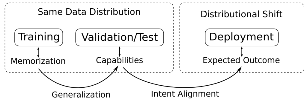
However, even when a model generalizes well to validation data, there is still a risk that its behavior will fail to align with human intentions when deployed in the real world. This is because the deployment environment may differ from the training and validation distributions in subtle but important ways. If the model has learned to rely on spurious correlations or shortcuts that happen to work in the training data but do not reflect the true underlying structure of the problem, it may exhibit unintended and potentially harmful behaviors when those correlations break down.
This is the essence of the inner alignment problem – ensuring that a system’s learned behavior not only generalizes to new data, but does so in a way that robustly captures the intended goals and values, even in the face of distributional shift and unanticipated situations. Solving this challenge requires going beyond simple generalization to validation data, and instead developing techniques for shaping a system’s learning process to be fundamentally aligned with human values.
In the rest of this post, we’ll explore one approach to tackling inner misalignment by framing it as a problem of identifying and mitigating harmful correlations in the learned features and decision-making process of an AI system. By better understanding these failure modes, we can work towards developing more robust and reliable techniques for value alignment.
Correlations
At the heart of the inner alignment problem is the issue of spurious correlations – patterns in the training data that are not causally related to the intended task, but which the model nevertheless learns to rely on. These correlations can lead to unintended and potentially harmful behaviors when the model is deployed in environments where those correlations no longer hold.
One striking example of this problem comes from the medical domain, as illustrated in figure below. In a study on skin lesion classification (Narla et al., 2018), researchers found that their model had learned to associate the presence of ruler markings with malignant tumors. This was because in the training data, which came from a hospital setting, rulers were more commonly used to measure concerning lesions. As a result, the model began to rely on the presence of rulers as a shortcut for identifying tumors, rather than learning the true underlying features of malignancy.
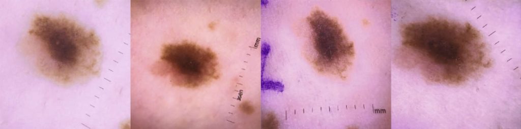
While this shortcut worked well on the validation set, which came from the same hospital distribution, it led to dangerous failures when the model was deployed on new data where rulers were not present. The model began to underestimate the prevalence of tumors, putting patients at risk. This illustrates how spurious correlations can lead to models that seem to perform well in validation, but fail to align with the intended behavior in deployment.
Another example of misalignment due to correlations comes from the realm of reinforcement learning, as shown in figure below. In this case, an agent was trained in a virtual environment to navigate to a goal (a coin) in order to receive a reward. The training environments always placed the coin in the far right corner of the level. As a result, the agent learned a policy of simply moving as far right as possible, rather than actually seeking out the coin.
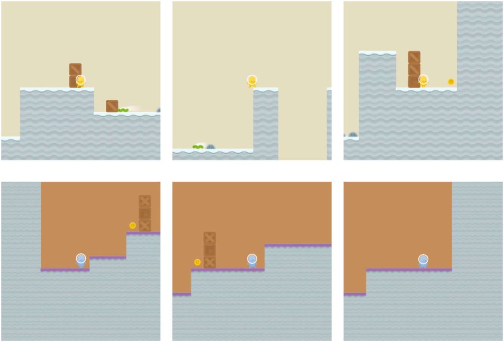
When deployed in new levels where the coin was placed in random locations, the agent continued to blindly move rightward, ignoring the coin even when it was right next to the agent’s starting position. This is because the agent had learned to optimize for the spurious correlation between rightward movement and reward, rather than learning the true goal of acquiring the coin.
These examples illustrate how correlations in the training data can lead to misaligned behavior in deployment, even when the model appears to perform well in validation. The key challenge is that these spurious correlations are often not easily identifiable to human auditors, as they may involve subtle statistical patterns in high-dimensional feature spaces.
This highlights the need for techniques to automatically identify and mitigate these harmful correlations during the learning process. By detecting when a model is relying on spurious features or exhibiting unintended behaviors, we can hope to intervene and guide the learning towards more robust and aligned representations. In the following section, we’ll explore a mathematical framework for doing just that, based on the idea of modeling the correlational structure of the learned features.
Mathematical Formulation
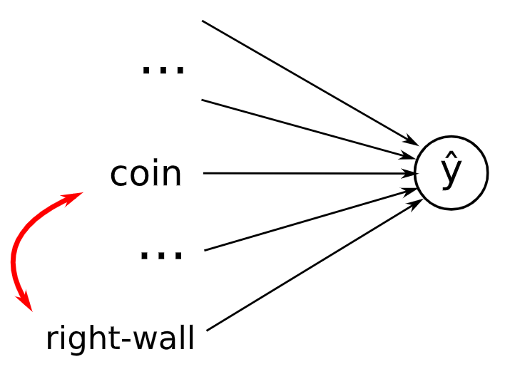
To tackle the problem of inner misalignment, we first need a way to characterize the distributions in which a model’s performance may be compromised due to spurious correlations. One approach is to start with a simple model, such as a single neuron or linear model, as depicted in the figure below. When such a model is trained on data with correlated features, it may learn to rely on these correlations in a way that fails to generalize to deployment environments where the correlations no longer hold.
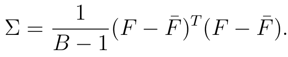
To capture these correlations mathematically, we can use the covariance matrix. The covariance matrix is a square matrix that represents the pairwise covariances between a set of features. For a set of D features, the covariance matrix has dimensions D x D, with each element (i, j) representing the covariance between the i-th and j-th features. The diagonal elements (i, i) represent the variances of each individual feature:
Intuitively, the covariance matrix allows us to identify correlated features by examining the patterns of covariance across the matrix. If two features i and j are highly correlated, they will have similar patterns of covariance with all other features, resulting in similar values across their corresponding rows and columns in the matrix.
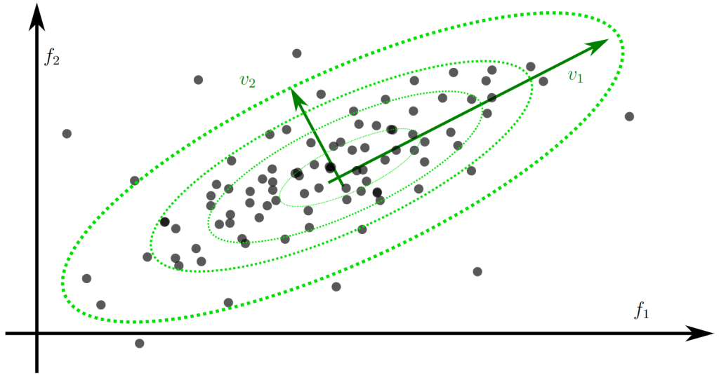
We can formalize this intuition using eigen decomposition. The eigenvectors of the covariance matrix represent the principal directions of variation in the data, with the corresponding eigenvalues indicating the amount of variance along each direction. Correlated features will have a principal direction (eigenvector) along which most of their variation occurs, and the corresponding eigenvalue will be large. Conversely, the eigenvectors with small eigenvalues represent directions in which the data varies the least, often corresponding to linear combinations of correlated features.
By projecting the original feature space onto these eigenvectors and scaling by the inverse square root of the eigenvalues, we arrive at the Mahalanobis distance. This is a distance metric that accounts for the correlational structure of the data, effectively normalizing the feature space so that distances are less sensitive to scaling and rotation.
The figure below illustrates these concepts visually. The ellipses represent contours of equal Mahalanobis distance from the mean of the data, with the eigenvectors v1 and v2 indicating the principal directions of variation. Points that are far apart in the original feature space may have a small Mahalanobis distance if they lie along a direction of high correlation, as the metric effectively compresses these correlated dimensions.
Mathematically, the Mahalanobis distance d(x) of a point x from the mean μ of a distribution with covariance matrix Σ is given by:
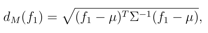
where T denotes the matrix transpose and -1 the matrix inverse. This distance can be seen as measuring the dissimilarity of a point from the center of a distribution, taking into account not just the individual feature values but their inter-relationships.
The Mahalanobis distance has a natural statistical interpretation as a measure of the probability density of a point under a multivariate Gaussian distribution. Points with a small Mahalanobis distance correspond to regions of high probability density, while points with a large distance correspond to low-density regions. This provides a principled way to identify points that are “atypical” or far from the training distribution, which may indicate a breakdown of the learned correlations and a risk of misaligned behavior.
By modeling the correlational structure of the learned features using covariance matrices and Mahalanobis distances, we can begin to develop techniques for automatically detecting and mitigating the risks of inner misalignment in deployment.
Implementation
To apply these ideas to more complex models, such as convolutional neural networks (CNNs), we need to adapt our approach to handle the high-dimensional, spatially structured feature maps learned by these architectures.
One straightforward approach is to flatten the feature maps into vectors and compute covariance matrices over these flattened representations. However, this discards the spatial structure of the features and can lead to very high-dimensional covariance matrices that are computationally challenging to work with, especially in the early layers of a deep network.
An alternative is to compute covariance matrices over local neighborhoods in the feature maps, such as 3×3 patches. This allows us to capture local correlations while preserving spatial structure and keeping the dimensionality manageable. Specifically, we can think of each local patch as a vector, and compute a shared covariance matrix over the set of all such patches in a given feature map. This covariance matrix then represents the local correlational structure of the features.
To compute the Mahalanobis distance for a new patch, we can flatten the patch into a vector, subtract the mean patch vector, and compute the quadratic form with the inverse covariance matrix as before. This operation can be efficiently implemented using convolution, by interpreting the inverse covariance matrix as a convolutional kernel.
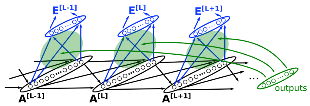
A further refinement of this approach is to compute class-conditional covariance matrices, rather than a single global covariance matrix. This is motivated by the observation that the correlational structure of features may vary depending on the class of the input. For example, in an object recognition task, the features indicative of a car may have a different correlational structure than those indicative of a person.
To implement this, we can compute separate covariance matrices for each class, conditioned on the output of the base model. That is, for each input, we first compute the model’s predicted class probabilities, and then use these probabilities to compute a weighted average of the class-conditional covariance matrices. This averaged covariance matrix is then used to compute the Mahalanobis distance for the input.
The figure below illustrates this idea, showing how the base model’s predictions are used to select and weight the class-conditional covariance matrices, which are then used to compute the Mahalanobis distance for each local patch. The distances are then aggregated (e.g., by averaging) to give an overall measure of the atypicality of the input.
One challenge with this approach is that the number of examples per class may be smaller than the dimensionality of the features, leading to rank-deficient or poorly conditioned covariance matrices. To mitigate this, we can regularize the covariance estimates by adding a small multiple of the identity matrix, ensuring that they remain invertible.
Another practical consideration is the memory and computation required to store and manipulate the covariance matrices, especially if the number of classes is large. To address this, we can use low-rank approximations or other compact representations of the covariance structure, such as diagonal or block-diagonal matrices.
Despite these challenges, the use of class-conditional covariance matrices and Mahalanobis distances offers a promising approach for detecting and mitigating the risks of inner misalignment in deep neural networks. By modeling the local correlational structure of the learned features in a class-aware way, we can identify inputs that deviate from the training distribution in a manner that is likely to lead to misaligned behaviors, and take corrective action.
For the implementation, we used a vectorized and incremental update code for calculating the mean and the covariance matrix for the features, eliminating the need for storing the activations over many batches and allowing a fast training of the detection modules.
Results
As both adversarial attacks and out-of-distribution data are the main vulnerabilities identified in the distributional shift and inner-misalignement that can be easily reproduced and testes, we address each of those individually.
Adversarial Attack Detection
To evaluate the effectiveness of our proposed methods in detecting adversarial attacks, we conducted experiments on the EfficientNetV2 model, which was pre-trained on the ImageNet dataset and fine-tuned on CIFAR-10. This modern CNN architecture, with its 21.5 million parameters, achieved over 97% accuracy on the CIFAR-10 dataset after fine-tuning.
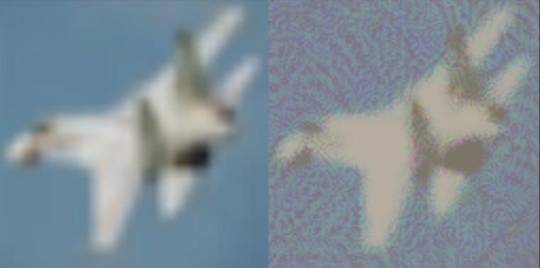
An interesting observation is that models pre-trained on larger datasets and then fine-tuned on smaller ones tend to be more robust to adversarial attacks compared to models trained solely on the smaller dataset. This robustness manifests in the larger magnitude of adversarial perturbation required to cause misclassification, as illustrated in the image below:
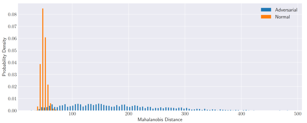
The figure below shows the distribution of Mahalanobis distances for the last Mahalanobis layer, which achieved the best classification performance between normal and adversarial samples. Normal samples are clustered on the left side of the histogram, with a mean of 48.6 and a standard deviation of 5.0 activation units, while adversarial samples have a mean of 174 and a standard deviation of 83 units. However, there are still some adversarial samples that exhibit similar activation metrics to normal samples, leading to potential misclassification.
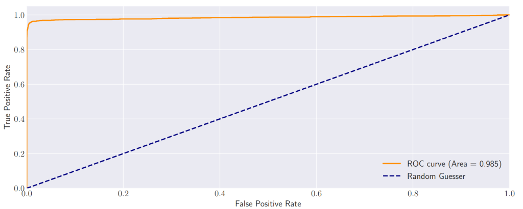
The Receiver Operating Characteristic (ROC) curve, depicted in below, better visualizes this behavior. By varying the classification threshold, we obtain different values for the True Positive Rate (TPR) and the False Positive Rate (FPR). The area under this curve (AUROC) serves as a single metric to compare different methods while capturing the tradeoff between the threshold value and the TPR and FPR. The last EBM achieved the highest AUROC value compared to the earlier layer EBMs, suggesting that the penultimate layer is the most salient for identifying adversarial attacks.
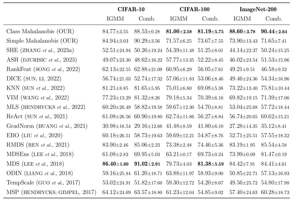
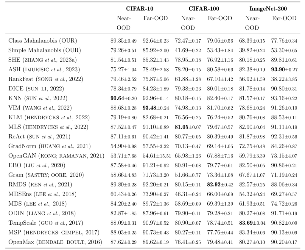
The table below presents the AUROC metrics for our proposed methods in comparison to other methods from the literature, as implemented in the OpenOOD framework. Our methods achieved the best results on the CIFAR-100 (tied with MDS) and ImageNet-200 datasets, and the second-best on CIFAR-10, with a small difference compared to the MDS method. While the Simple Mahalanobis method performs well on CIFAR-10, its single parametrization is insufficient to model the activation distributions as effectively as the Class Mahalanobis method on datasets with more output classes, such as CIFAR-100 and ImageNet-200. The IGMM is an Integrated Gradient method adversarial attack and the Comb. has both FGSM, BIM and PGD attacks.
These results demonstrate the potential of our proposed methods, particularly the Class Mahalanobis approach, in detecting adversarial attacks across various datasets and model architectures. By modeling the local correlational structure of learned features in a class-aware manner, we can identify inputs that deviate from the training distribution and are likely to cause misaligned behavior.
Out-Of-Distribution Detection
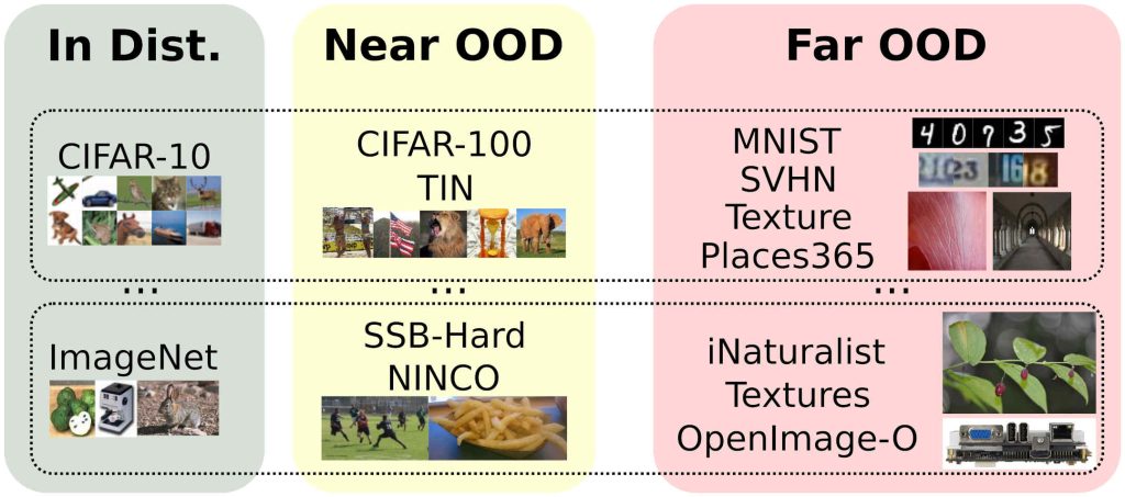
In addition to adversarial attack detection, we also evaluated our methods on the task of out-of-distribution (OOD) detection using the OpenOOD Benchmark. This benchmark is designed to assess OOD detection methods for image classification tasks on three main datasets: CIFAR-10, CIFAR-100, and ImageNet-1K.
The figure below provides a detailed view of the datasets that compose the OpenOOD Benchmark. For CIFAR-10, the official train set serves as the in-distribution (ID) training data, while a portion of the test set is held out for ID validation and testing. The near-OOD group includes CIFAR-100 and Tiny ImageNet (TIN), with some images removed due to overlap with CIFAR-10. The far-OOD group consists of MNIST, SVHN, Textures, and Places365. The CIFAR-100 benchmark follows a similar structure, with the same far-OOD group as CIFAR-10. For ImageNet-200, the near-OOD datasets are the Semantic Shift Benchmark (SSB) and NINCO (No ImageNet Class Objects), while the far-OOD datasets are Textures, OpenImage-O, and iNaturalist.
The table below presents the mean AUROC values and their standard deviations, calculated from three different instances of models with the same architecture, for the CIFAR-10, CIFAR-100, and ImageNet-200 OOD detection datasets. Our proposed methods did not achieve the best metrics in the benchmark, with the Simple Mahalanobis being effective only on CIFAR-10 and performing worse than a random classifier on the other datasets. However, the Class Mahalanobis method achieved the second-best result on CIFAR-10 and a median value on CIFAR-100.
The base model architectures used in the OpenOOD Benchmark are ResNet-18 models trained on CIFAR-10, CIFAR-100, and ImageNet-200 with fixed resolutions and standardized weights. These models were trained exclusively on the training subset of their respective datasets, initialized from random weights without transfer learning.
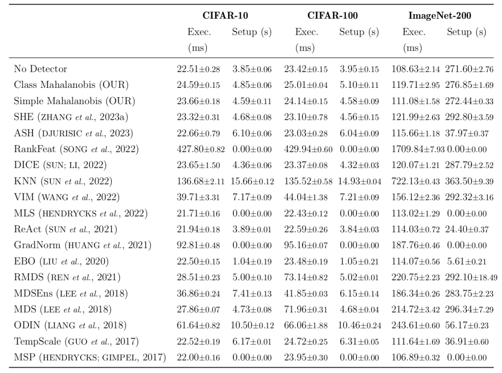
The Table below shows the mean execution and setup times for the OOD detection methods, along with their standard deviations. The execution time corresponds to the processing of a set of one thousand images during inference, while the setup time is the training time of the OOD detection models for one epoch of the validation data. Our methods had a very small overhead compared to the base model (No Detector), with less than a 10% increase in execution times, performing similarly to many other models.
These results highlight the challenges of OOD detection and the varying performance of our proposed methods across different datasets. While the Class Mahalanobis approach shows promise, particularly on CIFAR-10, there is still room for improvement in terms of generalization to more complex datasets like CIFAR-100 and ImageNet-200. The low overhead of our methods in terms of execution and setup times is encouraging, as it suggests that they can be integrated into existing models without significant computational burden.
Conclusions
In this blog post, we have explored the problem of inner misalignment in artificial intelligence systems, framing it as a challenge of identifying and mitigating harmful correlations in the learned features and decision-making processes of these models. We have seen how spurious correlations in training data can lead to models that exhibit unintended and potentially dangerous behaviors when deployed in real-world environments, even when they appear to perform well on validation data.
To address this issue, we have proposed two methods based on modeling the correlational structure of learned features using covariance matrices and Mahalanobis distances. The Simple Mahalanobis approach uses a single global covariance matrix to capture the overall feature correlations, while the Class Mahalanobis method employs class-conditional covariance matrices to model the feature correlations in a more fine-grained, class-aware manner.
We evaluated our methods on two critical tasks related to inner misalignment: adversarial attack detection and out-of-distribution detection. In the adversarial attack detection experiments, our Class Mahalanobis method demonstrated strong performance, achieving the best results on the CIFAR-100 and ImageNet-200 datasets and the second-best on CIFAR-10. These results suggest that modeling the local correlational structure of learned features in a class-aware fashion can effectively identify inputs that deviate from the training distribution and are likely to cause misaligned behavior.
On the out-of-distribution detection task, our methods showed mixed results. While the Class Mahalanobis approach performed well on CIFAR-10, achieving the second-best result, its performance on the more complex CIFAR-100 and ImageNet-200 datasets was less impressive. These findings underscore the challenges of generalizing OOD detection methods to diverse and challenging datasets.
Despite the varying performance across tasks and datasets, our methods demonstrated a notable advantage in terms of computational efficiency. The overhead introduced by our methods was minimal, with less than a 10% increase in execution times compared to the base models. This efficiency is crucial for the practical deployment of inner misalignment detection techniques in real-world systems.
In conclusion, our work highlights the importance of addressing inner misalignment in AI systems and proposes a promising approach based on modeling feature correlations. While our methods have shown encouraging results, particularly in adversarial attack detection, there remains significant room for improvement and further research. Future directions could include exploring more advanced techniques for modeling correlational structure, adapting the approach to better handle the complexity of larger datasets, and investigating the combination of our methods with other complementary techniques for inner misalignment detection and mitigation.
As AI systems continue to become more powerful and widely deployed, ensuring their alignment with human values and intentions is of paramount importance. By developing robust methods for detecting and correcting inner misalignment, we can work towards building AI systems that are more reliable, transparent, and beneficial to society as a whole.
Code Availability
The code is available in https://github.com/Gabrui/OpenOOD_Adv_Mahalanobis .
This blog post was prof-read with the help of Claude 2 and this work is also part of my PhD Thesis on AI Alignment that I am currently writing and that was also motivated by the course (I was previously working in a Computer Vision project but changed to AI Alignment).
Leave a Reply